The 6-s X-ray pulsar 1E1048.1-5937 was observed by EXOSAT in June 1985 for 20 ks. In this example, we'll conduct a general investigation of the spectrum from the Medium Energy (ME) instrument, i.e. follow the same sort of steps as the original investigators (Seward, Charles & Smale,1986). The ME spectrum and corresponding response matrix were obtained from the HEASARC On-line service.
Once installed, XSPEC is invoked by typing xspec, as in this example on rosserv, a Sun/4 workstation. The first command we issue is data followed by the name of the data file, e 1048_me.pha:
rosserv% xspec

                XSPEC 9.00 17:34:45 12-Jul-95

  Plot device not set, use "cpd" to set it

  Type "help" or "?" for further information
 XSPEC> data e1048_me.pha
 Net count rate (cts/cm^2/s) for file   1  2.2665E-03+/-  8.1922E-05
The data command tells the program to read the data as well as the response file that is named in the header of the data file. In general, XSPEC commands can be truncated, provided they remain unambiguous. Since the default extension of a data file is p.ha, the above command can be abbreviated to da e1048_me, if desired. To obtain help on the data command, or on any other command, type help command followed by the name of the command.
One of the first things most users will want to do at this stage-even before fitting models-is to look at their data. The plotting device should be set first, with the command cpd (change plotting device). Here, we use the Tektronix 4010 terminal emulator:
XSPEC> cpd /tek4010
To see a list of alternative plot devices, type cpd ? There are more than 20 different things that can be plotted, all related in some way to the data, the model, the fit and the instrument. To see them, type:
 XSPEC> plot ?
  Choose from the following `plot' sub-commands:
 data      counts    ldata     residuals chisq     delchi    ratio
 summary   contour   efficien  emodel    insensitv model     sensitvty
 ufspec    eufspec
 Insert selection: (data)
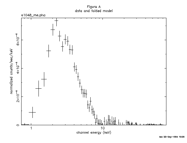
The most fundamental is the data plotted against instrument channel (data); next most fundamental, and more informative, is the data plotted against channel energy. To do this plot, use the XSPEC command setplot energy. Figure A shows the result of the commands:
 XSPEC> setplot energy
 XSPEC> plot data
People familiar with EXOSAT ME data will recognize the spectrum to be soft, absorbed and without an obvious bright iron emission line.
We are now ready to fit the data with a model. Models in XSPEC are specified using the model command, followed by a list of one or more model components chosen from the suite of more than seventy. There are two basic kinds of model: additive models which, after being convolved with the instrument response, prescribe the number of counts per energy bin (e.g., a bremsstrahlung continuum); and multiplicative models, which apply an energy-dependent multiplicative factor to additive models before convolution (e.g., an absorption edge). At least one additive component must be included in the model, but there is no restriction on the number of multiplicative models. To see what components are available, type model ? (for information about a specific component, type help model followed by the name of the component):
 XSPEC> model ?
  Possible additive models are :
  bbody    bbodyrad bknpower bremss   cemekl   cevmkl   cflow    compLS
  compST   compTT   cp6mkl   cp6vmkl  cutoffpl disk     diskbb   diskline
  diskm    disko    gaussian meka     mekal    mkcflow  nteea    pegpwrlw
  pexrav   pexriv   pliref   plrefl   powerlaw raymond  redge    step
  tita_a   useradd1 vbremss  vmeka    vmekal   vmcflow  vraymond zbbody
  zbremss  zgauss   zplrefl  zpowerlw atable
  Possible multiplicative models are :
  absori   constant cabs     cyclabs  dust     edge     expabs   expfac
  highecut hrefl    notch    pcfabs   phabs    plabs    smedge   spline
  SSS_ice  usermul1 uvred    varabs   wabs     wndabs   zedge    zhighect
  zpcfabs  zphabs   zvarabs  zvfeabs  zwabs    zwndabs  mtable   etable
  Possible mixing models are :
  ascac
Given the quality of our data, as shown by the plot, we'll choose an absorbed power law, specified as follows :
XSPEC> model wabs powerlaw
Or, abbreviating unambiguously:
XSPEC> mo wa po
Either way, the user is prompted straight away for the initial values of the parameters. Hitting return in response to a prompt enters the default values. As well as the parameter values themselves, users also may specify step sizes and ranges (value, delta, min, bot, top, and max values), but here, we'll enter the defaults:
  mo = wabs[1] (powerlaw[2])
 Input parameter value, delta, min, bot, top, and max values for ...
 Mod parameter  1 of component  1  1 wabs     nH 10^22
    1.000      1.0000E-03      0.          0.      1.0000E+05  1.0000E+06

 Mod parameter  2 of component  2  1 powerlaw PhoIndex
    1.000      1.0000E-02  -10.00      -9.000       9.000       10.00

 Mod parameter  3 of component  2  0 powerlaw norm
    1.000      1.0000E-03      0.          0.      1.0000E+05  1.0000E+06

   ---------------------------------------------------------------------------
   ---------------------------------------------------------------------------
   mo = wabs[1] (powerlaw[2])
   Model Fit Model   Component     Parameter   Value
   par   par comp
     1    1    1       wabs        nH 10^22   1.00000     +/-      0.
     2    2    2       powerlaw    PhoIndex   1.00000     +/-      0.
     3    3    2       powerlaw    norm       1.00000     +/-      0.
   ---------------------------------------------------------------------------
   ---------------------------------------------------------------------------
     3 variable fit parameters
  Chi-Squared =     4.9092E+08 using   125 PHA bins.
  Reduced chi-squared =     4.0239E+06
The Çurrent statistic is  and is huge for the initial,
default values-mostly because the power law normalization is two
orders of magnitude too large. This is easily fixed using the
renorm command :
and is huge for the initial,
default values-mostly because the power law normalization is two
orders of magnitude too large. This is easily fixed using the
renorm command :
 XSPEC> ren
  Chi-Squared =      840.5     using   125 PHA bins.
  Reduced chi-squared =      6.890
We are not quite ready to fit the data (and obtain a better
), because not all of the 125 PHA
bins should be included in the fitting: some are below the lower
discriminator of the instrument and therefore do not contain valid data;
some have negative count rates because of imperfect background
subtraction at the margins of the pass band; and some may not contain
enough counts for to be strictly meaningful. To find out
which channels to discard (ignore in XSPEC terminology),
users must consult mission-specific documentation, which will inform them
of discriminator settings, background subtraction problems and other
issues. For the mature missions in the HEASARC archives, this
information already has been encoded in the headers of the spectral
files as a list of ``bad" channels. Simply issue the command:
 XSPEC> ignore bad
  Chi-Squared =      788.1     using    85 PHA bins.
  Reduced chi-squared =      9.611
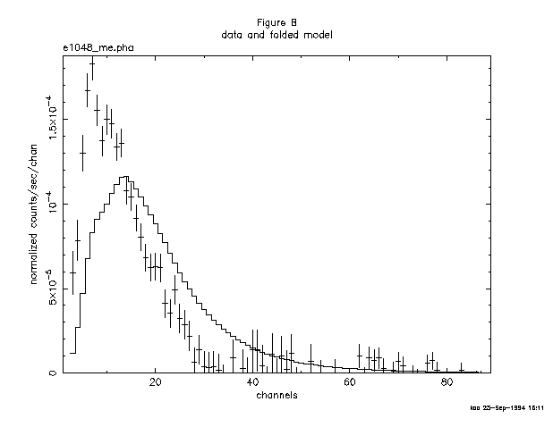
We can see that 40 channels are bad-but do we need to ignore any more? These channels are bad because of certain instrument properties: other channels still may need to be ignored because of the shape and brightness of the spectrum itself. Figure B shows the result of plotting the data in channels (using the commands setplot channel and plot data). We see that the channels above channel 33 start to contain negative counts. We also see, comparing Figure B with Figure A, which bad channels were ignored. Although visual inspection is not the most rigorous method for deciding which channels to ignore (more on this subject later), it's good enough for now, and will at least prevent us from getting grossly misleading results from the fitting. To ignore channels above 33:
 XSPEC> ignore 34-**
  Chi-Squared =      666.0     using    31 PHA bins.
  Reduced chi-squared =      23.79
The same result can be achieved with the command ignore 34-125. The inverse of ignore is notice, which has the same syntax.
We are now ready to fit the data. Fitting is initiated by the command
fit. As the fit proceeds, the screen displays the status of the
fit for each iteration until either the fit converges to the minimum
, or the user is asked whether the fit is to go through
another set of iterations to find the minimum. The default number of
iterations is ten, but in our example, convergence is attained after
eight:
 XSPEC> fit
  Chi-Squared  Lvl  Fit param # 1     2           3
    288.68     -4         0.       2.188      8.1403E-03
    48.264     -5         0.       1.914      8.5292E-03
    33.220     -6         0.       1.995      8.8701E-03
    33.214     -7         0.       1.996      8.8726E-03
    32.930      0     3.7669E-02   1.996      8.8858E-03
    32.591     -1     6.9828E-02   2.001      9.0296E-03
    31.325     -2     0.2030       2.062      9.8992E-03
    30.753     -3     0.4391       2.172      1.1650E-02
    30.022     -4     0.5011       2.198      1.2305E-02
 Number of trials exceeded - last iteration delta =   0.7311
  Continue fitting? (Y)
    30.014     -5     0.5037       2.199      1.2338E-02
   ---------------------------------------------------------------------------
   ---------------------------------------------------------------------------
   mo = wabs[1] (powerlaw[2])
   Model Fit Model   Component     Parameter   Value
   par   par comp
     1    1    1       wabs        nH 10^22  0.503747     +/- 0.29087
     2    2    2       powerlaw    PhoIndex   2.19871     +/- 0.12856
     3    3    2       powerlaw    norm      1.233789E-02 +/- 0.24629E-02
   ---------------------------------------------------------------------------
   ---------------------------------------------------------------------------
  Chi-Squared =      30.01     using    31 PHA bins.
  Reduced chi-squared =      1.072
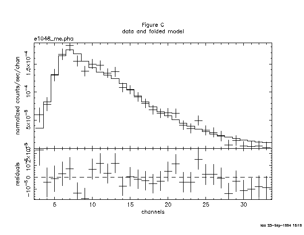
The fit is good: reduced is 1.072 for 31 - 3 = 29 degrees of
freedom. To see the fit and the residuals, we can use the command
plot data resid. The result is shown in Figure C.
The screen output shows the best-fitting parameter values, as well as approximations to their errors. These errors should be regarded as indications of the uncertainties in the parameters and should not be quoted in publications. The true errors, i.e. the confidence ranges, are obtained using the error command:
 XSPEC> error 1 2 3
  Fit Index   Confidence Range (     2.706)
      1    3.934827E-02     1.01198
      2     1.99501         2.41692
  *WARNING*:RENORM: No variable model to allow renormalization
  *WARNING*:RENORM: No variable model to allow renormalization
  *WARNING*:RENORM: No variable model to allow renormalization
  *WARNING*:RENORM: No variable model to allow renormalization
  *WARNING*:RENORM: No variable model to allow renormalization
  *WARNING*:RENORM: No variable model to allow renormalization
  *WARNING*:RENORM: No variable model to allow renormalization
  *WARNING*:RENORM: No variable model to allow renormalization
  *WARNING*:RENORM: No variable model to allow renormalization
  *WARNING*:RENORM: No variable model to allow renormalization
      3    8.963043E-03    1.734988E-02
Here, the numbers 1, 2, 3 refer to the parameter numbers in the Fit
par column of the screen output. For the first parameter, the column of
absorbing hydrogen atoms, the 90% confidence range is  cm
cm . This corresponds to an
excursion in of 2.706. The reason these ``better" errors are
not given automatically as part of the fit output is that they
entail further fitting. When the model is simple, this does not require
much CPU, but for complicated models the extra time can be
considerable. The warning message is generated because there are
no free normalizations in the model while the error is being
calculated on the normalization itself. In this case, the warning may
safely be ignored.
. This corresponds to an
excursion in of 2.706. The reason these ``better" errors are
not given automatically as part of the fit output is that they
entail further fitting. When the model is simple, this does not require
much CPU, but for complicated models the extra time can be
considerable. The warning message is generated because there are
no free normalizations in the model while the error is being
calculated on the normalization itself. In this case, the warning may
safely be ignored.
What else can we do with the fit? One thing is to derive the flux of the model. The data by themselves only give the instrument-dependent count rate. The model, on the other hand, is an estimate of the true spectrum emitted. In XSPEC, the model is defined in physical units independent of the instrument. The command flux integrates the current model over the range specified by the user:
 XSPEC> flux 2 10
  Model flux 3.5488E-03 photons (2.2489E-11 ergs)cm**-2 s**-1 (  2.000- 10.000)
Here, we have chosen the standard X-ray range of 2-10 keV and find that
the energy flux is  erg cm s
 . Note
that flux will integrate only within the energy range of the
current response matrix. If the model flux outside this range is
desired-in effect, an extrapolation beyond the data-then the command
dummyrsp should be used. This command reads in a dummy response
that covers the range required. For example, if we want to know the flux
of our model in the ROSAT PSPC band of 0.2-2 keV, we enter:
. Note
that flux will integrate only within the energy range of the
current response matrix. If the model flux outside this range is
desired-in effect, an extrapolation beyond the data-then the command
dummyrsp should be used. This command reads in a dummy response
that covers the range required. For example, if we want to know the flux
of our model in the ROSAT PSPC band of 0.2-2 keV, we enter:
 XSPEC> dummyrsp 0.2 2
  Chi-Squared =      3586.     using    31 PHA bins.
  Reduced chi-squared =      128.1
 XSPEC> flux 0.2 2
  Model flux 4.4267E-03 photons (8.9990E-12 ergs)cm**-2 s**-1 (  0.200-  2.000)
The energy flux, at  erg cm s, is
lower in this band but the photon flux is higher. To get our original
response matrix back we enter :
erg cm s, is
lower in this band but the photon flux is higher. To get our original
response matrix back we enter :
 XSPEC> response
  Chi-Squared =      30.01     using    31 PHA bins.
  Reduced chi-squared =      1.072
The fit, as we've remarked, is good, and the parameters are constrained. But unless the purpose of our investigation is merely to measure a photon index, it's a good idea to check whether alternative models can fit the data just as well. We also should derive upper limits to components such as iron emission lines and additional continua, which, although not evident in the data nor required for a good fit, are nevertheless important to constrain. First, let's try an absorbed black body:
 XSPEC> mo wa bb
  mo = wabs[1] (bbody[2])
 Input parameter value, delta, min, bot, top, and max values for ...
 Mod parameter  1 of component  1 wabs     nH 10^22
    1.000      1.0000E-03      0.          0.      1.0000E+05  1.0000E+06

 Mod parameter  2 of component  2 bbody    kT(keV)
    3.000      1.0000E-02  1.0000E-04  1.0000E-02   100.0       200.0

 Mod parameter  3 of component  2 bbody    norm
    1.000      1.0000E-03      0.          0.      1.0000E+05  1.0000E+06

   ---------------------------------------------------------------------------
   ---------------------------------------------------------------------------
   mo = wabs[1] (bbody[2])
   Model Fit Model   Component     Parameter   Value
   par   par comp
     1    1    1       wabs        nH 10^22   1.00000     +/-      0.
     2    2    2       bbody       kT(keV)    3.00000     +/-      0.
     3    3    2       bbody       norm       1.00000     +/-      0.
   ---------------------------------------------------------------------------
   ---------------------------------------------------------------------------
     3 variable fit parameters
  Chi-Squared =     3.3333E+09 using    31 PHA bins.
  Reduced chi-squared =     1.1905E+08
 XSPEC> fit
  Chi-Squared  Lvl  Fit param # 1     2           3
    1103.2     -1         0.       1.925      3.0014E-04
    789.99     -1         0.      0.7774      1.5796E-04
    374.84     -2         0.      0.9160      3.5594E-04
    174.80     -3         0.      0.9008      2.4199E-04
    136.09     -4         0.      0.8922      3.0098E-04
    120.19     -5         0.      0.8914      2.6655E-04
    115.88     -6         0.      0.8912      2.8554E-04
    114.38     -7         0.      0.8911      2.7471E-04
    113.92     -8         0.      0.8911      2.8078E-04
 Number of trials exceeded - last iteration delta =   0.4537
  Continue fitting? (Y)
    113.78     -9         0.      0.8911      2.7734E-04
    113.73    -10         0.      0.8911      2.7928E-04
    113.71    -11         0.      0.8911      2.7818E-04
    113.71    -12         0.      0.8911      2.7880E-04
    113.71      0         0.      0.8913      2.7859E-04
   ---------------------------------------------------------------------------
   ---------------------------------------------------------------------------
   mo = wabs[1] (bbody[2])
   Model Fit Model   Component     Parameter   Value
   par   par comp
     1    1    1       wabs        nH 10^22        0.     +/- -1.0000
     2    2    2       bbody       kT(keV)   0.891259     +/- 0.16956E-01
     3    3    2       bbody       norm      2.785949E-04 +/- 0.74475E-05
   ---------------------------------------------------------------------------
   ---------------------------------------------------------------------------
  Chi-Squared =      113.7     using    31 PHA bins.
  Reduced chi-squared =      4.061
Note that when more than 10 iterations are required for convergence the user is asked whether or not to continue at the end of each set of 10. Saying no at these prompts is a good idea if the fit is not converging quickly. Conversely, to avoid having to keep answering the question, i.e., to increase the number of iterations before the prompting question appears, begin the fit with, say:
XSPEC> fit 100
This command will put the fit through 100 iterations before pausing.
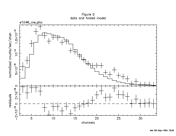
The black body fit is obviously not a good one. Not only is
large, but the best-fitting  is rather low. Inspection of the
residuals confirms this: the pronounced wave-like shape is indicative of
a bad choice of overall continuum (see Figure D). Let's try thermal
bremsstrahlung next:
is rather low. Inspection of the
residuals confirms this: the pronounced wave-like shape is indicative of
a bad choice of overall continuum (see Figure D). Let's try thermal
bremsstrahlung next:
 XSPEC> mo wa br
  mo = wabs[1] (bremss[2])
 Input parameter value, delta, min, bot, top, and max values for ...
 Mod parameter  1 of component  1 wabs     nH 10^22
    1.000      1.0000E-03      0.          0.      1.0000E+05  1.0000E+06

 Mod parameter  2 of component  2 bremss   kT(keV)
    7.000      5.0000E-02  0.1000       1.000       100.0       200.0

 Mod parameter  3 of component  2 bremss   norm
    1.000      1.0000E-03      0.          0.      1.0000E+05  1.0000E+06

   ---------------------------------------------------------------------------
   ---------------------------------------------------------------------------
   mo = wabs[1] (bremss[2])
   Model Fit Model   Component     Parameter   Value
   par   par comp
     1    1    1       wabs        nH 10^22   1.00000     +/-      0.
     2    2    2       bremss      kT(keV)    7.00000     +/-      0.
     3    3    2       bremss      norm       1.00000     +/-      0.
   ---------------------------------------------------------------------------
   ---------------------------------------------------------------------------
     3 variable fit parameters
  Chi-Squared =     3.2534E+08 using    31 PHA bins.
  Reduced chi-squared =     1.1619E+07
 XSPEC> fit
  Chi-Squared  Lvl  Fit param # 1     2           3
    42.435     -4         0.       5.087      3.5213E-03
    27.906     -5         0.       5.373      3.5658E-03
    27.906     -6         0.       5.370      3.5687E-03
    27.906      1         0.       5.370      3.5687E-03
   ---------------------------------------------------------------------------
   ---------------------------------------------------------------------------
   mo = wabs[1] (bremss[2])
   Model Fit Model   Component     Parameter   Value
   par   par comp
     1    1    1       wabs        nH 10^22        0.     +/- -1.0000
     2    2    2       bremss      kT(keV)    5.36973     +/- 0.41151
     3    3    2       bremss      norm      3.568679E-03 +/- 0.26339E-03
   ---------------------------------------------------------------------------
   ---------------------------------------------------------------------------
  Chi-Squared =      27.91     using    31 PHA bins.
  Reduced chi-squared =     0.9966
Bremsstrahlung is a better fit than the black body-and is as good as
the power law-although it shares the low . With two good fits,
the power law and the bremsstrahlung, it's time to scrutinize their
parameters in more detail.
From the EXOSAT database on HEASARC, we know that the target in
question, 1E1048.1-5937, has a Galactic latitude of 24 arcmin, i.e.,
almost on the plane of the Galaxy. In fact, the data base also provides
the value of the Galactic based on 21-cm radio observations. At
 cm, it is higher than the 90 percent-confidence upper
limit from the power-law fit. Perhaps, then, the power-law fit is not so
good after all. What we can do is fix (freeze in XSPEC
terminology) the value of at the Galactic value and refit the
power law. Although we won't get a good fit, the shape of the residuals
might give us a clue to what is missing. To freeze a parameter in
XSPEC, use the command freeze followed by the parameter number,
like this:
cm, it is higher than the 90 percent-confidence upper
limit from the power-law fit. Perhaps, then, the power-law fit is not so
good after all. What we can do is fix (freeze in XSPEC
terminology) the value of at the Galactic value and refit the
power law. Although we won't get a good fit, the shape of the residuals
might give us a clue to what is missing. To freeze a parameter in
XSPEC, use the command freeze followed by the parameter number,
like this:
 XSPEC> freeze 1
 Number of variable fit parameters =    2
The inverse of freeze is thaw:
 XSPEC> thaw 1
 Number of variable fit parameters =    3
Alternatively, parameters can be frozen using the newpar command,
which allows all the quantities associated with a parameter to be
changed. The second quantity, delta, is the step size used in the
fitting, and, if set to a negative number, will cause the parameter to
be frozen. In our case, we want frozen at
cm, so we go back to the power law best fit
and do the following :
 XSPEC> newpar 1
 Input parameter value, delta, min, bot, top, and max values for ...
 Mod parameter  1 of component  1 wabs     nH 10^22
   0.5038      1.0000E-03      0.          0.      1.0000E+05  1.0000E+06
 4,0
   ---------------------------------------------------------------------------
   ---------------------------------------------------------------------------
   mo = wabs[1] (powerlaw[2])
   Model Fit Model   Component     Parameter   Value
   par   par comp
     1    1    1       wabs        nH 10^22   4.00000     frozen
     2    2    2       powerlaw    PhoIndex   2.19872     +/- 0.12856
     3    3    2       powerlaw    norm      1.233807E-02 +/- 0.24628E-02
   ---------------------------------------------------------------------------
   ---------------------------------------------------------------------------
     2 variable fit parameters
  Chi-Squared =      776.6     using    31 PHA bins.
  Reduced chi-squared =      26.78
Note the useful trick of giving a value of zero for delta in the newpar command. This has the effect of changing zero to the negative of its current value. If the parameter is free, it will be frozen, and if frozen, thawed. The same result can be obtained by putting everything onto the command line, i.e., newpar 1 4, 0, or by issuing the two commands, newpar 1 4 followed by freeze 1. Now, if we fit again, we get the following set of parameters:
   ---------------------------------------------------------------------------
   ---------------------------------------------------------------------------
   mo = wabs[1] (powerlaw[2])
   Model Fit Model   Component     Parameter   Value
   par   par comp
     1    1    1       wabs        nH 10^22   4.00000     frozen
     2    2    2       powerlaw    PhoIndex   3.51070     +/- 0.66531E-01
     3    3    2       powerlaw    norm      0.102057     +/- 0.81193E-02
   ---------------------------------------------------------------------------
   ---------------------------------------------------------------------------
  Chi-Squared =      113.6     using    31 PHA bins.
  Reduced chi-squared =      3.916
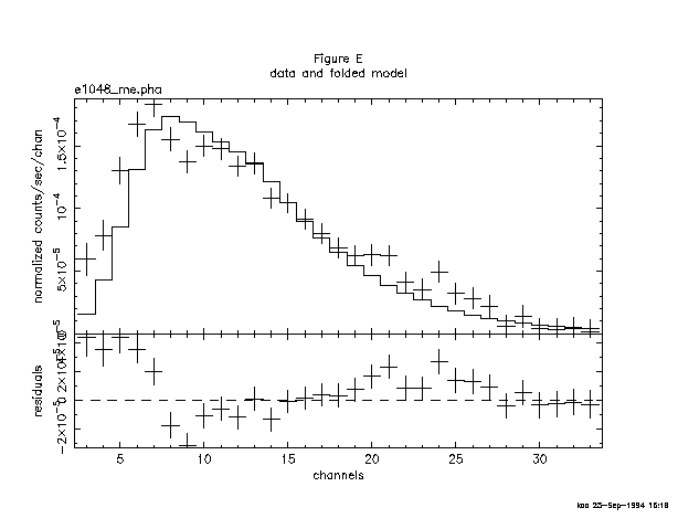
The fit is not good. In Figure E we can see why: there appears to be a surplus of softer photons, perhaps indicating a second continuum component. To investigate this possibility we can add a component to our model. The addcomp command lets us do this without having to respecify the model from scratch. Here, we'll add a black body component. The numerical argument of addcomp is the component number, which indicates where in the model the component should go. Thus, addcomp 3 bb will add a black body after the power law:
 XSPEC> addcomp 3 bb
 Input parameter value, delta, min, bot, top, and max values for ...
 Mod parameter  4 of component  3 bbody    kT(keV)
    3.000      1.0000E-02  1.0000E-04  1.0000E-02   100.0       200.0
 2,0
 Mod parameter  5 of component  3 bbody    norm
    1.000      1.0000E-03      0.          0.      1.0000E+05  1.0000E+06
 1.e-5
   ---------------------------------------------------------------------------
   ---------------------------------------------------------------------------
   mo = wabs[1] (powerlaw[2] + bbody[3])
   Model Fit Model   Component     Parameter   Value
   par   par comp
     1    1    1       wabs        nH 10^22   4.00000     frozen
     2    2    2       powerlaw    PhoIndex   3.51070     +/- 0.66531E-01
     3    3    2       powerlaw    norm      0.102057     +/- 0.81193E-02
     4    4    3       bbody       kT(keV)    2.00000     frozen
     5    5    3       bbody       norm      1.000000E-05 +/-      0.
   ---------------------------------------------------------------------------
   ---------------------------------------------------------------------------
     3 variable fit parameters
  Chi-Squared =      110.6     using    31 PHA bins.
  Reduced chi-squared =      3.948
Notice that in specifying the initial values of the black body, we have frozen kT at 2 keV (the canonical temperature for nuclear burning on the surface of a neutron star in a low-mass X-ray binary) and started the normalization at zero. Without these measures, the fit might ``lose its way". Notice, too, the line in the screen output that indicates where the command (addcomp 3) placed the blackbody, mo = wabs[1] (powerlaw[2] + bbody[3]). Now, if we fit, we get (not showing all the iterations this time):
   ---------------------------------------------------------------------------
   ---------------------------------------------------------------------------
   mo = wabs[1] (powerlaw[2] + bbody[3])
   Model Fit Model   Component     Parameter   Value
   par   par comp
     1    1    1       wabs        nH 10^22   4.00000     frozen
     2    2    2       powerlaw    PhoIndex   4.76352     +/- 0.15957
     3    3    2       powerlaw    norm      0.303830     +/- 0.43608E-01
     4    4    3       bbody       kT(keV)    2.00000     frozen
     5    5    3       bbody       norm      2.275169E-04 +/- 0.34069E-04
   ---------------------------------------------------------------------------
   ---------------------------------------------------------------------------
  Chi-Squared =      51.84     using    31 PHA bins.
  Reduced chi-squared =      1.851
The fit is better than the one with just a power law and the fixed Galactic column, but it is still not good. Thawing the black body temperature and fitting gives us:
   ---------------------------------------------------------------------------
   ---------------------------------------------------------------------------
   mo = wabs[1] (powerlaw[2] + bbody[3])
   Model Fit Model   Component     Parameter   Value
   par   par comp
     1    1    1       wabs        nH 10^22   4.00000     frozen
     2    2    2       powerlaw    PhoIndex   6.12218     +/- 0.38323
     3    3    2       powerlaw    norm      0.801310     +/- 0.22076
     4    4    3       bbody       kT(keV)    1.21930     +/- 0.87138E-01
     5    5    3       bbody       norm      2.592895E-04 +/- 0.28472E-04
   ---------------------------------------------------------------------------
   ---------------------------------------------------------------------------
  Chi-Squared =      35.61     using    31 PHA bins.
  Reduced chi-squared =      1.319
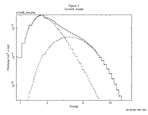
This, of course, is a better fit, but the photon index of the power law has ended up extremely and implausibly steep. Looking at this odd model (with the command plot model), we see, in Figure F, that the black body and the power law have changed places, in that the power law provides the soft photons required by the high absorption, while the black body provides the harder photons.
We could continue to search for a plausible, well-fitting model, but the data, with their limited signal-to-noise and energy resolution, probably don't warrant it (the original investigators published only the power law fit). There is, however, one final, useful thing to do with the data: derive an upper limit to the presence of a fluorescent iron emission line. First we delete the black body component using the inverse of addcomp, namely, delcomp:
 XSPEC> delcomp 3
   mo = wabs[1] (powerlaw[2])
  Chi-Squared =      1236.     using    31 PHA bins.
  Reduced chi-squared =      42.62
Then we thaw and refit to recover our original, best fit (output
not shown). Then, we add a gaussian emission line of fixed energy and
width:
 XSPEC> addcomp 3 gaussian
 Input parameter value, delta, min, bot, top, and max values for ...
 Mod parameter  4 of component  3 gaussian LineE
    6.500      5.0000E-02      0.          0.       100.0       100.0
 6.4 0
 Mod parameter  5 of component  3 gaussian Sigma
   0.1000      5.0000E-02      0.          0.       10.00       20.00
 ,0
 Mod parameter  6 of component  3 gaussian norm
    1.000      1.0000E-03      0.          0.      1.0000E+05  1.0000E+06
 1.e-4
   ---------------------------------------------------------------------------
   ---------------------------------------------------------------------------
   mo = wabs[1] (powerlaw[2] + gaussian[3])
   Model Fit Model   Component     Parameter   Value
   par   par comp
     1    1    1       wabs        nH 10^22  0.504116     +/- 0.29075
     2    2    2       powerlaw    PhoIndex   2.19884     +/- 0.12845
     3    3    2       powerlaw    norm      1.234063E-02 +/- 0.24683E-02
     4    4    3       gaussian    LineE      6.40000     frozen
     5    5    3       gaussian    Sigma     0.100000     frozen
     6    6    3       gaussian    norm      1.000000E-04 +/-      0.
   ---------------------------------------------------------------------------
   ---------------------------------------------------------------------------
     4 variable fit parameters
  Chi-Squared =      32.64     using    31 PHA bins.
  Reduced chi-squared =      1.209
The energy and width have to be frozen because,in the absence of an obvious line in the data, the fit would be completely unable to converge on meaningful values. Besides, our aim is to see how bright a line at 6.4 keV can be and still not ruin the fit. To do this, we fit first and then use the error command to derive the maximum allowable iron line normalization. We then set the normalization at this maximum value with newpar and, finally, derive the equivalent width using the eqwidth command. That is:
 XSPEC> err 6
  Fit Index   Confidence Range (     2.706)
  Parameter pegged at hard limit         0.
  with delta ftstat=     1.800
      6          0.        1.421908E-04
 XSPEC> new 6 1.421908E-04
     4 variable fit parameters
  Chi-Squared =      33.25     using    31 PHA bins.
  Reduced chi-squared =      1.231
 XSPEC> eqwidth 3
  Additive group equiv width for model 3 (gaussian): 780. eV
Things to note:
 of 2.706 when the minimum value hit zero, the ``hard"
lower limit of the parameter. Hard limits can be adjusted with the
newpar command, and they correspond to the quantities min
and max associated with the parameter values. In fact, according
to the screen output, the value of corresponding to zero
normalization is 1.805.
of 2.706 when the minimum value hit zero, the ``hard"
lower limit of the parameter. Hard limits can be adjusted with the
newpar command, and they correspond to the quantities min
and max associated with the parameter values. In fact, according
to the screen output, the value of corresponding to zero
normalization is 1.805.